Implementing Bit-addressing with Specialization
Scott Draves
School of Computer Science
Carnegie Mellon University
5000 Forbes Avenue, Pittsburgh, PA 15213,
USA
hardcopy -
references -
appendix -
thanks
to appear in ICFP97
Abstract
General media-processing programs are easily expressed with
bit-addressing and variable-sized bit-fields. But the natural
implementation of bit-addressing relies on dynamic shift offsets and
repeated loads, resulting in slow execution. If the code is
specialized to the alignment of the data against word boundaries, the
offsets become static and many repeated loads can be removed. We show
how introducing modular arithmetic into an automatic compiler
generator enables the transformation of a program that uses
bit-addressing into a synthesizer of fast specialized programs.
In partial-evaluation jargon we say: modular arithmetic is supported
by extending the binding time lattice used by the static analysis in a
polyvariant compiler generator. The new binding time  functions
like a partially static integer.
functions
like a partially static integer.
A software cache combined with a fast, optimistic sharing analysis
built into the compilers eliminates repeated loads and stores. The
utility of the transformation is demonstrated with a collection of
examples and benchmark data. The examples include vector arithmetic,
audio synthesis, image processing, and a base-64 codec.
Introduction
Media such as audio, images, and video are increasingly common in
computer systems. Such data are represented by large arrays of small
integers known as samples. Rather than wasting bits, samples are
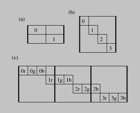
packed into memory. Figure combined illustrates three
examples: monaural sound stored as an array of 16-bit values, a
grayscale image stored as an array of 8-bit values, and a color image
stored as interleaved 8-bit arrays of red, green, and blue samples.
Such arrays are called signals.
 ps
ps
Figure combined: Layout of (a) 16-bit
monaural sound, (b) an 8-bit grayscale image, and (c) a 24-bit color
image. The heavy lines indicate 32-bit word boundaries.
Say we specify a signal's representation with four integers: from
and to are bit addresses; size and stride are numbers of
bits. We use `little-endian' addressing so the least significant bit
of each word (LSB) has the least address of the bits in that word.
type signal = int * int * int * int
           (* from  to    size  stride *)
Figure sig-sum gives the code to sum the elements of a signal.
This and other examples use ML syntax extended with infix bit
operations as found in the C programming language (<< >> & |). The
load_word primitive accesses a memory location. This paper
assumes 32-bit words, but any other size could just as easily be
substituted even at run-time. The integer division (/) rounds
toward minus infinity; integer remainder (%) has positive base and
result. To simplify this presentation, load_sample does not
handle samples that cross word boundaries.
fun sum (from, to, size, stride) r =
  if from = to then r else
  sum ((from+stride), to, size, stride)
      (r + (load_sample from size))

fun load_sample p b =
   ((1 << b) - 1) &
   ((load_word (p / 32)) >> (p % 32))
Figure sig-sum:
Summing a signal using bit addressing.
If we fix the layout by assuming stride = size = 8 and (from %
32) = (to % 32) = 0 then the implementation in Figure sig-sum-fast computes the same value, but runs more than five times
faster (see Figure table3). There are several reasons: the
loop is unrolled four times, resulting in fewer conditionals and more
instruction level parallelism; the shift offsets and masks are known
statically, allowing immediate-mode instruction selection; the
division and remainder computations in load_sample are avoided;
redundant loads are eliminated.
fun sum_0088 from to r =
  if from = to then r else
  let val v = load_word from
  in sum_0088 (from + 1) to
    (r + (v & 255) + ((v >> 8) & 255) +
    ((v >> 16) & 255)+ ((v >> 24) & 255))
  end
Figure sig-sum-fast:
Summing a signal assuming packed, aligned 8-bit samples as in Figure
combined(b).
Different assumptions result in different code. For example,
sequential 12-bit samples result in unrolling 8=lcm(12,32)/12 times so
that three whole words are loaded each iteration (see Figure twelve). Handling samples that cross word boundaries requires adding
a conditional to load_sample that loads an additional word, then
does a shift-mask-shift-or sequence of operations.
 ps
ps
Figure twelve:
12-bit signal against 32-bit words shown with abbreviated vertical
axis.
As such, the programmer is faced with a familiar trade-off: write one
slow, easy-to-read, general-purpose routine; or write many fast
special cases. We pursue an alternative: write general-purpose code
and automatically derive fast special cases. The techniques presented
here are designed to be fast enough to generate special cases lazily
at run-time, thus providing an interface to run-time code generation
(RTCG). It is not strictly necessary that specialization occur at
run-time, but because the number of special cases is exponential in
the number of static arguments, code space quickly becomes a problem
if the specialization is all done at compile time, as with macro and
C++ template expansion.
As a concrete example consider the screen position of a window. The
horizontal coordinate affects the alignment of its pixels against the
words of memory, so special-purpose graphics operations may be created
each time a window is opened or moved. As another example, consider
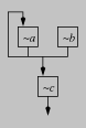
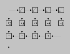
an interactive audio designer. A particular `voice' is defined by a
small program; Figure fm is a typical example of an FM
synthesizer. Most systems allow the user to pick from several
predefined voices and adjust their scalar parameters. With RTCG, the
user may define voices with their own wiring diagrams.
 ps
ps  ps
ps
Figure fm: Two voices.
On the left is a simple 2-in-1 FM synthesizer. Oscillators a and
b sum to modulate c as well as feeding back into a. On
the right is another possibility.
Other interfaces to run-time code generation have been explored in a
variety of places: there have been manual systems such as Common Lisp
[Steele90] with eval, macros with backquote/comma syntax, and
slow code generation. Fast manual systems such as Synthesis [Massalin92] and the Blit terminal [PiLoRei85] confirmed the
performance benefits of RTCG in operating systems and bit-mapped
graphics, respectively. `C [EnHsKa95] adds a Lisp-style
interface to RTCG to the C programming language. Fabius [LeLe96]
uses fast automatic specialization for run-time code generation of a
subset of ML, but cannot handle bit-addressing. Tempo [CoHoNoNoVo96] attempts to automate the kind of RTCG used by Synthesis.
Self takes an automatic but less general approach to run-time code
generation [ChaUng91], as do recent just-in-time (JIT)
implementations of Java [GoJoSte96].
Past work in bit-level processing has not emphasized implementation on
word-machines. VHDL [IEEE91] allows this level of specification,
but lacks an efficient compiler. Synchronous real-time languages like
Signal [GuBoGaMa91] support programming with streams, but not at
the bit level.
This paper shows how to implement bit-addressing with a partial
evaluator.
Section spec presents a polyvariant, direct-style specializer
and briefly describes how to derive a compiler generator from it.
Section cyclic extends the specializer with cyclic integers,
resulting in an analysis similar to [Granger89]. Section irregular shows how irregular (data-dependent) layouts are handled.
Section loads shows how extending of partial evaluation allows
fast elimination of redundant loads and stores. Section impls
describes two implementations of these ideas; Section eg
presents example source programs and compares the performance of the
generated code with hand-written C programs.
Specialization
We begin our discussion of specialization with a definition, then we
introduce our notation and give a simple polyvariant specializer for a
 -language. Section cogen discusses efficient
implementation via compiler generaton and introduces the concept of
binding times. Section spec is generally a review of partial
evaluation practice; [JoGoSe93] is the standard text of the field
and may be considered a reference of first resort if you can find it.
[WeiCoRuSe91] is a more widely available description of an
advanced on-line specializer. The system described here is a
polyvariant version of type-directed partial evaluation [Danvy96], much like [Sheard96].
-language. Section cogen discusses efficient
implementation via compiler generaton and introduces the concept of
binding times. Section spec is generally a review of partial
evaluation practice; [JoGoSe93] is the standard text of the field
and may be considered a reference of first resort if you can find it.
[WeiCoRuSe91] is a more widely available description of an
advanced on-line specializer. The system described here is a
polyvariant version of type-directed partial evaluation [Danvy96], much like [Sheard96].
A specializer  satisfies the following equation where italic
names denote program texts and Quine quotes
satisfies the following equation where italic
names denote program texts and Quine quotes ![{\\tt{}[\\negthinspace{}\\negthinspace{}[$\\cdot$]\\negthinspace{}\\negthinspace{}]}](3.gif) denote ordinary evaluation:
denote ordinary evaluation: ![\\begin{code}[\\negthinspace{}\\negthinspace{}[$f$]\\negthinspace{}\\negthinspace{}] $x$ $y$ = [\\negthinspace{}\\negthinspace{}[[\\negthinspace{}\\negthinspace{}[$mix$]\\negthinspace{}\\negthinspace{}] $f$ {\\tt{}} $x$]\\negthinspace{}\\negthinspace{}] $y$\\end{code}](4.gif)
There are many ways to implement ![{\\tt{}[\\negthinspace{}\\negthinspace{}[$mix$]\\negthinspace{}\\negthinspace{}]}](5.gif) ; a simple curry function suffices. Our intension is that
will do as much work of
; a simple curry function suffices. Our intension is that
will do as much work of  as is possible knowing only its first argument and return a residual program that finishes the computation. Because we expect to
use this residual function many times, this gives us a way of
`factoring' or `staging' computations as in [JoSche86].
as is possible knowing only its first argument and return a residual program that finishes the computation. Because we expect to
use this residual function many times, this gives us a way of
`factoring' or `staging' computations as in [JoSche86].
Figure domains gives the grammar of our object language, and
defines some domains and their metavariables. The language is the
-calculus extended with explicit types on abstractions,
constants, primitives, a conditional, and a lift annotation.
We say the lift is an `annotation' because in the `ordinary' semantics
of the -calculus, lift has no meaning; it becomes the identity
function. The ordinary semantics can be useful for debugging.
Figure specf gives a specializer  . The notation
![{\\tt{}[$v$$\\mapsto$$k$]}$\\rho$](8.gif) denotes updating the
environment
denotes updating the
environment  with a binding from the variable
  to the value
  ;
;  denotes a generic, `black box' binary primitive
operation;
denotes a generic, `black box' binary primitive
operation;  mark manipulation of the terms of the
-language's syntax (like Lisp's backquote);
mark manipulation of the terms of the
-language's syntax (like Lisp's backquote);  denotes pattern matching
where the metavariables only match the appropriate domain.
denotes pattern matching
where the metavariables only match the appropriate domain.
Figure helpers defines the reification and reflection
functions  and
and  . They operate as coercions between code and
data; understanding them is not essential to this work.
. They operate as coercions between code and
data; understanding them is not essential to this work.
is a partial-evaluation function; it assigns a meaning
from  to a source text with environment. The difference from an
ordinary semantics is that contains
to a source text with environment. The difference from an
ordinary semantics is that contains  , whose members represent
computations dependent on unknown values, i.e. are residual code. We
say the specializer emits residual code.
, whose members represent
computations dependent on unknown values, i.e. are residual code. We
say the specializer emits residual code.
We say is polyvariant because a given piece of syntax may
be both executed by and emitted as residual. This happens to
f in this example:
let fun f x = x + 1
    fun g s d = (f s) + (f d)
in (g 1 (lift 1))
end
Creating general code and a special case of the same source text
corresponds to the standard `fast-path' optimization technique.
Note that the if clause requires that when a conditional has
dynamic predicate, then both arms are also dynamic.
is similar to the -mix of [GoJo91], but because
-mix is monovariant, it uses a two-level input language where
source lambda terms have been labeled either for execution or
immediate residualization. reserves judgement until the
is applied; depends on lift annotations to emit
functions.
Note that many cases are missing from . We assume that all
input programs are type-correct and lift annotations appear as
necessary. Placement of the lifts is crucial to successful staging:
too many lifts and degenerates into the curry function; too few
and fails to terminate. Typically binding time analysis
(BTA) is combined with programmer annotations to insert the lifts.
For example, if =[a-->6 b--> ]
] then
requires ((lift a)b) rather than (ab). This kind of lift is obvious, and is easily handled
by BTA. As an example of the kind of lift that cannot be
easily automated, consider the following tail-recursive function:
fun loop b e r =
  if (1 = e) then r
  else loop b (e - 1) (b * r)
fun power b e = loop b e 1
where e is in and b is in  . Unless we manually
lift
. Unless we manually
lift r to dynamic, will diverge.
Monovariant BTA is well-understood and can be efficiently implemented
with type-inference [Henglein91]. Polyvariant BTA is usually
implemented with abstract interpretation [Consel93].

Figure domains:
The -language, domains and metavariables. is a
primitive;  is the set of variables.
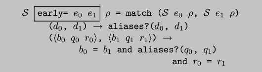
![\\begin{code*}$\\cal{}S$ : $\\sf{}Exp$ $\\times$ $\\sf{}Env$ $\\rightarrow$ $\\sf{}M$
\\codeskip
$\\cal{}S$ \\fbox{$e_0$$\\diamond$$e_1$} $\\rho$ = match ($\\cal{}S$ $e_0$ $\\rho$, $\\cal{}S$ $e_1$ $\\rho$)
($s_0$, $s_1$) $\\rightarrow$ $s_0$ $\\diamond$ $s_1$
($d_0$, $d_1$) $\\rightarrow$ \\fbox{$d_0$ $\\diamond$ $d_1$}
$\\cal{}S$ \\fbox{$v$} $\\rho$ = $\\rho$ $v$
$\\cal{}S$ \\fbox{$k$} $\\rho$ = $k$
$\\cal{}S$ \\fbox{lambda $v$:$t$.$e$} $\\rho$ =
($\\lambda$$v'$.$\\cal{}S$ $e$ ([$v$$\\mapsto$$v'$]$\\rho$))${}_t$
$\\cal{}S$ \\fbox{$e_0$ $e_1$} $\\rho$ = match ($\\cal{}S$ $e_0$ $\\rho$, $\\cal{}S$ $e_1$ $\\rho$)
($f$, $m$) $\\rightarrow$ $f$ $m$
($d_0$, $d_1$) $\\rightarrow$ \\fbox{$d_0$ $d_1$}
$\\cal{}S$ \\fbox{lift $e$} $\\rho$ = $R$ ($\\cal{}S$ $e$ $\\rho$)
$\\cal{}S$ \\fbox{if $e_0$ $e_1$ $e_2$} $\\rho$ =
match ($\\cal{}S$ $e_0$ $\\rho$)
$s_0$ $\\rightarrow$ if $s_0$ then ($\\cal{}S$ $e_1$ $\\rho$)
else ($\\cal{}S$ $e_2$ $\\rho$)
$d_0$ $\\rightarrow$ let $d_1$ = $\\cal{}S$ $e_1$ $\\rho$
$d_2$ = $\\cal{}S$ $e_2$ $\\rho$
in \\fbox{if $d_0$ then $d_1$ else $d_2$}
end
\\end{code*}](23.gif)
Figure specf:
A direct-style polyvariant specializer.

Figure helpers:
Reification function and reflection function .
can be defined with like this:
![\\begin{code}[\\negthinspace{}\\negthinspace{}[$mix$]\\negthinspace{}\\negthinspace{}] $e$ $x$ = $R$([\\negthinspace{}\\negthinspace{}[$R$([\\negthinspace{}\\negthinspace{}[$R$($\\cal{}S$ $e$ [])]\\negthinspace{}\\negthinspace{}] $x$)]\\negthinspace{}\\negthinspace{}] \\fbox{y})
\\end{code}](25.gif) but this is just a hypothetical and rather limited way to access
.
but this is just a hypothetical and rather limited way to access
.
Now we return to the sum example to see the result of
specializing it without cyclic values. Conceptually[footnote: Not
formally because our -language is not the ML of the example.],
we specialize the text of sum to its size and stride like
this:
![\\begin{code}$\\cal{}S$ $sum$ [from$\\rightarrow$\\fbox{from} to$\\rightarrow$\\fbox{to}
size$\\rightarrow$8 stride$\\rightarrow$8 r$\\rightarrow$\\fbox{r}]\\end{code}](26.gif) In the residual code, the mask computation
In the residual code, the mask computation ((1 << b) - 1) becomes
constant, but all other operations are unaffected.
Compiler Generation
If we use a literal implementation of to specialize programs,
then every time we generate a residual program, we also traverse and
dispatch on the source text. The standard way to avoid this repeated
work is to introduce another stage of computation, that is, to use a
compiler generator cogen instead of a specializer mix. The
compiler generator converts into a synthesizer of specialized
versions of :
![\\begin{code}[\\negthinspace{}\\negthinspace{}[$f$]\\negthinspace{}\\negthinspace{}] $x$ $y$ = [\\negthinspace{}\\negthinspace{}[[\\negthinspace{}\\negthinspace{}[[\\negthinspace{}\\negthinspace{}[$cogen$]\\negthinspace{}\\negthinspace{}] $f$]\\negthinspace{}\\negthinspace{}] $x$]\\negthinspace{}\\negthinspace{}] $y$
\\end{code}](27.gif)
These systems are called compiler generators because if is an
interpreter, then ![{\\tt{}[\\negthinspace{}\\negthinspace{}[$cogen$]\\negthinspace{}\\negthinspace{}]$f$}](28.gif) is a compiler;
the part of the execution of we call `interpretation overhead'
is only performed once. Although a procedure like
is a compiler;
the part of the execution of we call `interpretation overhead'
is only performed once. Although a procedure like sum is not what
we normally think of as an interpreter, the idea is the same:
factoring-out the overhead of using a general representation.
The standard way of implementing a compiler generator begins with a
static analysis of the program text, then produces the synthesizer by
syntax-directed traversal of the text annotated with the results of
the analysis. Cogen knows what will be constant but not the constants
themselves. We call such information binding times; they
correspond to the injection tags on a members of . We say members
of are static and members of are dynamic. The
binding times form a lattice because they represent partial
information: it is always safe for the compiler to throw away
information; this is called lifting and is the meaning of the lift annotation in the -language.
[BoDu93] shows how to derive a cogen from -mix in two
steps. The first step converts a specializer into a compiler
generator by adding an extra level of quoting to so static
statements are copied into the compiler and dynamic ones are emitted.
The second step involves adding a continuation argument to to
allow propagation of a static context into the arms of a conditional
with a dynamic test. One of the interesting results of [Danvy96]
is how this property (the handling of sum-types) can be achieved while
remaining in direct style by using the shift/reset control operators
([DaFi92] Section 5.2).
Making a working implementation of a compiler generator in a
call-by-value language requires handling of memoization, inlining, and
code duplication as well. Practical systems usually supply heuristics
and syntax to control these features. Many systems (including ours)
use the dynamic-conditional heuristic, which inlines calls to
procedures that do not contain a conditional with dynamic predicate.
A remarkably pleasing though less practical way of implementing
![{\\tt{}[\\negthinspace{}\\negthinspace{}[$cogen$]\\negthinspace{}\\negthinspace{}]}](29.gif) is by self-application of a
specializer
is by self-application of a
specializer ![{\\tt{}[\\negthinspace{}\\negthinspace{}[[\\negthinspace{}\\negthinspace{}[$mix$]\\negthinspace{}\\negthinspace{}] $mix$ $mix$]\\negthinspace{}\\negthinspace{}]}](30.gif) , as suggested in [Futamura71] and first
implemented in [JoSeSo85].
, as suggested in [Futamura71] and first
implemented in [JoSeSo85].
Cyclic Integers
This section shows how adding some rules of modular arithmetic to the
compiler generator can unroll loops, make shift offsets static, and
eliminate the division and remainder operations inside the load_sample procedure.
Figure domains2 defines the domain, redefines to
include as a possible meaning, and extends to handle cyclic
values. Whereas previously an integer value was either static or
dynamic (either known or unknown), a cyclic value has known base and
remainder but unknown quotient. The base must be positive. Initially
we assume the remainder is `normal', ie non-negative and less than the
base.
Figure addmult0 gives an initial version of the addition and
multiplication cases for on cyclic values. Again we assume
cases not given are avoided by lifting, treating the primitives as
unknown (allowing to match any primitive), or by using the
commutivity of the primitives. The multiplication rule doesn't handle
negative scales. A case for adding two cyclic values by taking the
GCD of the bases is straightforward, but has so far proven
unnecessary. Such multiplication is also possible, though more
complicated and less useful.
Note that this addition rule contains a dynamic addition to the
quotient. But in many cases  is zero; so the addition may be
omitted up by the backend (GCC handles this fine). But the allocation
of a new dynamic location would confuse the sharing analysis (see
Section loads). Furthermore, The multiplication rule has its
own defect: in order to maintain normal form we must dissallow
negative scales.
is zero; so the addition may be
omitted up by the backend (GCC handles this fine). But the allocation
of a new dynamic location would confuse the sharing analysis (see
Section loads). Furthermore, The multiplication rule has its
own defect: in order to maintain normal form we must dissallow
negative scales.
The rules used by Nitrous appear in Figure addmult1. They are
simpler and more general because Nitrous imposes normal form only at
memoization points.
Figure domains2:
Extending domains and for cyclic values.

Figure addmult0: First attempt at extending to cyclic values; normal form is
maintained.

Figure addmult1: Rules for addition and multiplication.
Figure spec3:
More rules for cyclic values.
Figure spec3 gives rules for zero?, division, and
remainder. These rules are interesting because the binding time of
the results depends on the static value rather than just the binding
times of the arguments as in the previous rules. In the case of zero?, if the remainder is non-zero, then we can statically conclude
that the original value is non-zero. But if the remainder is zero,
then we need a dynamic test of the quotient. This is a conjunction
short-circuiting across stages, and is why we require a polyvariant
system. If we constrain such tests to be immediately consumed by a
conditional, then one could probably incorporate these techniques into
a monovariant system.
Division and remainder could also use polyvariance, but experience
indicates this is expensive and is not essential, so our systems just
raise an error.
Instead of adding rules to the specializer, we could get some of the
same functionality by defining (in the object language) a new type
which is just a partially static structure with three members. The
rules in Figures addmult0 and spec3 become procedures
operating on this type. This has the advantage of working with an
ordinary specializer, but the disadvanage of not interacting well with
sharing.
Now we explain the impact of cyclic values on the sum
example. The result of
![\\begin{code}$\\cal{}S$ $sum$ [from$\\rightarrow$$\\langle$32 \\fbox{fromq} 0$\\rangle$ to$\\rightarrow$$\\langle$32 \\fbox{toq} 0$\\rangle$
size$\\rightarrow$8 stride$\\rightarrow$8 r$\\rightarrow$\\fbox{r}]\\end{code}](36.gif) appears in Figure resid1. Because the loop index is cyclic
three equality tests are done in the compiler before it reaches an
even word boundary. At this point, the specializer emits a dynamic
test and forms the loop. Note that
appears in Figure resid1. Because the loop index is cyclic
three equality tests are done in the compiler before it reaches an
even word boundary. At this point, the specializer emits a dynamic
test and forms the loop. Note that fromq and toq are
word-pointers.
If the alignments of from and to had differed, then the `odd'
iterations would have been handled specially before entering the
loop. The generation of this prelude code is a natural and automatic
result of using cyclic values; normally it is generated by hand or by
special-purpose code in a compiler.
If we want to apply this optimization to a dynamic value, then we can
use case analysis to convert it to cyclic before the loop, resulting in
one prelude for each possible remainder, followed by a single loop.
fun sum_0088 fromq toq r =
   if fromq = toq then r else
     sum_0088 (fromq + 1) to
      (r+(((load_word fromq)>>0)&255) +
          (((load_word fromq)>>8)&255) +
          (((load_word fromq)>>16)&255) +
          (((load_word fromq)>>24)&255))
Figure resid1:
Residual code automatically generated with cyclic values.
Arbitrary arithmetic on pointers could result in values with any base,
but once we are in a loop like sum we want a particular base.
set-base gives the programmer control:
 Since
Since  may be dynamic,
 set-base can be used to perform case
analysis. While we currently rely on manual placement of set-base, we believe automation is possible.
Multiple Signals
If a loop reads from multiple signals simultaneously then it must be
unrolled until all the signals return to their original alignment.
The ordinary way of implementing a pair-wise operation on same-length
signals uses one conditional in the loop because when one vector ends,
so does the other. Since our unrolling depends on the conditional,
this would result in the alignments of one of the vectors being
ignored.
To solve this, we perform such operations with what normally would be
a redundant conjunction of the end-tests. In both implementations the
residual loop has only one conditional, though after it exits it makes
one redundant test[footnote: Nitrous does this because it uses
continuations; Simple does because its compiler to C translates while(E&&F)S to while(E)while(F)S.]. Figure binop
illustrates this kind of loop.
Because 32 has only one prime factor (2), on 32-bit machines this
conjunction amounts to taking the worst case of all of the signals.
If the word-size were composite then more complex cases could occur,
for example, 24-bit words with signals of stride 8 and 12 results in
unrolling 6 times.
fun binop (from, to, size, stride)
          (from', to', size', stride') =
   if ((from = to) andalso (from' = to'))
   then ()
   else (... ; binop( ... ))
Figure binop:
Looping over two signals.
Irregular Data Layout
The sum example shows how signals represented as simple arrays can
be handled. The situation is more complex when the data layout
depends on dynamic values. Examples of this include sparse matrix
representations, run length encoding, and strings with escape
sequences. Figure escape shows how 15-bit values might be
encoded into an 8-bit stream while keeping the shift offsets static.
It works because both sides of the conditional of v are
specialized.
Read_esc is a good example of the failure of the
dynamic-conditional heuristic. Unless we mark the recursive call as
dynamic (so it is not inlined), specialization would diverge because
some strings are never aligned, as illustrated in Figure escape2.
fun read_esc from to r =
  if from = to then r
  else let val v = load_sample from 8
    in if (v < 128)
      then read_esc (from + 8) to (next v r)
       else d@ read_esc (from+16) to
       (next (((v & 127) << 8) |
        (load_sample (from + 8) 8)) r)
    end
Figure escape:
Reading a string of 8-bit characters with escape sequences. d@
indicates a dynamic call.
 ps
ps
Figure escape2: A string with escapes
illustrating need for dynamic call annotation in read_esc.
Sharing and Caching
The remaining inefficiency of the code in Figure resid1 stems
from the repeated loads. The standard approach to eliminating them is
to apply common subexpression elimination (CSE) and aliasing analysis
(see Chapter 10.8 of [ASeUl86]) to residual programs. Efficient
handling of stores is beyond traditional techniques, however. We
propose fast, optimistic sharing and static caching as an alternative.
We implement the cache with a monad [Wadler92]. Uses of the load_word primitive are replaced by calls to a cached load procedure
load_word_c. The last several addresses and memory values are
stored in a table in the monad; when load_word_c is called the
table is checked. If a matching address is found, the previously
loaded value is returned, otherwise memory is referenced, a new table
entry is created, and the least recently used table entry is
discarded. Part of the implementation appears in Appendix A. In fact,
any cache strategy could be used as long as it does not depend on the
values themselves.
Note that safely eliminating loads in the presence of stores requires
negative may-alias information (knowing that values will not be equal)
[Deutsch94]. We have not yet implemented anything to guarantee
this.
The prime variable is the size of the cache. How many previous loads
should be stored? Though this is currently left to a manual setting,
automation appears feasible because requirements combine simply.
How does the cache work? Since the addresses are dynamic any kind of
equality test of the addresses will be dynamic. Yet these tests must
be static if the cache is to be eliminated. Our solution is to use a
conservative early equality operator for the cache-hit tests:
 This operator takes two dynamic values and returns a static value; the
compiler returns true only if it can prove the values will be equal,
this is positive alias (sharing) information. The aliasing
information becomes part of the static information given to compilers,
stored in the memo tables, etc. Details appear in [Draves96].
This operator takes two dynamic values and returns a static value; the
compiler returns true only if it can prove the values will be equal,
this is positive alias (sharing) information. The aliasing
information becomes part of the static information given to compilers,
stored in the memo tables, etc. Details appear in [Draves96].
In Nitrous the generated compilers keep track of the names of the
dynamic values; the aliases? function merely tests these names for
equality. Thus at compile time a cached load operation requires only
a set-membership (memq) operation. These names are also used for
inlining without a postpass (among other things), so no additional
work is required to support early=. Simple uses textual equality
of the terms.
The cache functions like a CSE routine specialized to examine only
loads, so we expect a cache-based compiler to run faster than a
CSE-based one. But since CSE subsumes the use of a cache and is
probably essential to good performance anyway, why do we consider the
cache? Because CSE cannot handle stores, but the cache does, as
explained below.
Like the optimizations of the previous section, these load
optimizations have been achieved by making the compiler generator more
powerful (supporting early=). Even more so than the previous
section, the source program had to be written to take advantage of
this. Fortunately, with the possible exception of cache size, the
modifications can be hidden behind ordinary abstraction barriers.
Store Caching
So far we have only considered reading from memory, not writing to it.
Storing samples is more complicated than loading for two reasons: an
isolated store requires a load as well as a store, and optimizing
stores most naturally requires information to move backwards in time.
This is because if we read several words from the same location, then
the reads after the first are redundant. But if we store several
words to the same location, all writes before the last write are
redundant.
We can implement store_word_c the same way a hardware write-back
cache does (second edition of [HePa90] page 379): cache lines are
extended with a dirty flag; stores only go to memory when a cache line
is discarded. The time problem above is solved by buffering the
writes.
The load is unnecessary if subsequent stores eventually overwrite the
entire word. Solving this problem requires extending the
functionality of the cache to include not just dirty lines, but
partially dirty lines. Thus the status of a line may be either clean
or a mask indicating which bits are dirty and which are not present in
the cache at all. When a line is flushed, if it is clean no action is
required. If it is dirty and the mask is zero, then the word is
simply stored. Otherwise a word is fetched from memory, bit-anded
with the mask, bit-ored with the line contents, and written to memory.
Implementations
We currently have two implementations of bit-addressing: Nitrous and
Simple, a first-order system. Both are available from http://www.cs.cmu.edu/~spot.
Nitrous [Draves96] is an automatic compiler generator for a
higher-order, three-address-code intermediate language. It handles
partially-static structures (product types), moves static contexts
past dynamic conditionals (sum types), cyclic integers, sharing, and
memoization. It uses the dynamic-conditional heuristic. Cache and
signal libraries were implemented in a high-level language and
compiled to the intermediate language[footnote: In fact, this
compilation was performed with a generated compiler as well; the
output of the output of cogen is fed into cogen.].
A number of examples were specialized, compiled to C (including GCC's
indirect-goto extension), and benchmarked. At the time of [Draves96], performance was about half that of hand-written,
specialized C code; since then the performance has been significantly
improved.
Unfortunately Nitrous fails to terminate when given more complicated
input. The reason is unknown, but we suspect exponential static
code is being generated as a result of the aggressive propagation
of static data, particularly in the cache and inside nested loops.
In order to scale-up the examples, we built Simple, an on-line
specializer that avoids using shift/reset or continuations by
restricting dynamic control flow to loops (ie sum and arrow types are
not fully handled). It is a straight-forward translation of the
formal system presented in this paper. All procedure calls in the
source programs are expanded, but the input language is extended with
a while-loop construct that may be residualized:
 which is equivalent to the following simple recursive procedure:

The loop construct is specialized as if it were a recursive procedure
with the dynamic conditional heuristic and memoization:
it is inlined until the predicate is dynamic, then the loop is entered
and unrolled until the predicate is dynamic again. At this point, the
static part must match the static part at the previous dynamic
conditional.
Because Simple is based on symbolic expansion, code is duplicated in
the output of the specializer. GCC's optimizer fixes most of these.
The specializer is written in SML/NJ without concern for speed but the
examples here specialize in fractions of a second.
Example
The main example built with the simple system is an audio/vector
library. It provides the signal type, constructors that create
signals from scalars or sections of memory, combinators such as
creating a signal that is the sum of two other signals, and
destructors such as copy and reduce. The vector operations are
suspended in constructed data until a destructor is called. Figure
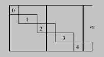
fir contains a graphical representation of this kind of
program.
 ps
ps
Figure fir: A graphical `tinker-toy' DSP program. z is a delay.
Interleaved vectors are stored in the same range of memory; Figure
combined(c) is an example of three interleaved vectors. With
an ordinary vector package, if one were to pass interleaved vectors to
a binary operation, then each input word would be read twice. A
on-chip hardware cache makes this second read relatively
inexpensive. But with the software cache the situation is detected once at code-generation time; specialization replaces a cache hit
with a register reference.
Figure sig gives the signature for part of the library. The
semantics and implementation are mostly trivial; some of the code
appears in Appendix B. One exception is that operations on multiple
signals use a conjunction on the end test (Section multiple). As a corollary, endp of an infinite signal such as a
constant always returns true.
The delay operator returns a signal of the same length as its input,
thus it loses the last sample of the input signal. The other
possibility (that it returns a signal one longer) requires sum-types
because there would be a dynamic conditional in the next method.
The filter combinator is built out of a series of delays, maps, and
binops. Another combinator built from combinators is the FM
oscillator.
Simple uses first-order analogues of the higher-order arguments. We
can implement recursive filters (loops in the dataflow) with state, as
wavrec, scan, and delay1 do. A higher-order system would
support a general purpose rec operator for creating any recursive
program.
sig
  type samp
  type signal
  type address
  type binop = samp * samp -> samp

  fun get: signal -> samp
  fun put: signal -> samp -> unit
  fun next: signal -> signal
  fun endp: signal -> bool

  fun memory: address * address
            * int * int -> signal
  fun constant: samp -> signal

  fun map: (samp -> samp) * signal -> signal
  fun map2: binop * signal * signal -> signal
  fun delay1: signal * samp -> signal
  fun scan: signal * samp * binop -> signal
  fun lut: address * signal -> signal
  fun sum_tile: samp * signal * int -> signal

  fun copy: signal * signal -> unit
  fun reduce: signal * samp * binop -> samp

  fun filter: signal * (samp * samp) list
               -> signal
  fun fm_osc: signal * int * address * int *
              signal * int -> signal
end
Figure sig:
Signature for signal library.
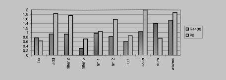
The benchmarks were performed by translating the specialized code to C
and compiling with GCC v2.7.2 with the -O1 option. We also collected
data with the -O2 option, but it was not significantly different so we
do not present it. O3 is not available on our SGI. There are two
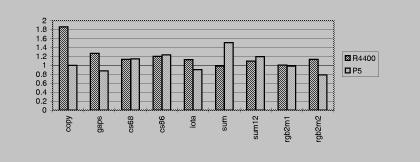
groups of examples, the audio group (Figure table1) and the
video group (Figure table2). The audio group uses 2000-byte
buffers and 16-bit signals; the video group uses 4000-byte buffers and
mostly 8-bit signals.
Each of the examples was run for 1000 iterations; real elapsed time
was measured with the gettimeofday system call. The whole suite
was run five times, and the best times were taken. The R4400 system
is an SGI Indigo with 150Mhz R4400 running IRIX 5.3. The P5 is
an IBM Thinkpad 560 with 133Mhz Pentium running Linux 2.0.27.
with 150Mhz R4400 running IRIX 5.3. The P5 is
an IBM Thinkpad 560 with 133Mhz Pentium running Linux 2.0.27.
The graphs show the ratio of the execution time of the code generated
by Simple to manually written C code. In the audio group, this code
was written using short* pointers and processing one sample per
iteration. In the video group, the code was written using whole-word
memory operations and immediate-mode shifts/masks. Some of the code
appears in Appendix manual.
Some of the static information used to create the specialized loops
appears in Appendix benche. These are generally arguments to
the `interpreter' copy, which is used for all the audio examples.
The video examples also use copy, except iota, sum, and sum12.
The audio examples operate on sequential aligned 16-bit data unless
noted otherwise:
- inc
- add 10 to each sample.
- add
- two signals to form a third.
- filter2
- filter with kernel width 2.
- filter5
- filter with kernel width 5. The manual code doesn't
unroll the inner loop over the kernel.
- fm 1
- a one oscillator FM synthesizer.
- fm 2
- a one-in-one oscillator FM synthesizer.
- lut
- a look-up table of size 256. The input signal is 8-bits per
pixel.
- sum
- all the samples in the input
- wavrec
- an FM synthesizer with feedback.
The video examples operate on sequential aligned 8-bit data unless
noted otherwise:
- copy
- no operation.
- gaps
- destination signal has stride 16 and size 8.
- cs68
- converts binary to ASCII by reading a six-bit signal and
writing eight.
- cs86
- ASCII to binary by reading eight and writing six.
- iota
- fills bytes with 0, 1, 2, ...
- sum
- as in Figure sig-sum, specialized as in Figure sig-sum-fast
- sum12
- a twelve-bit signal.
 ps
ps
Figure table1: Audio group. Speed
of automatically generated code normalized to speed of
hand-specialized code.
 ps
ps
Figure table2: Video group. Speed
of automatically generated code normalized to speed of
hand-specialized code.
 ps
ps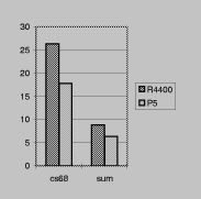 ps
ps
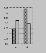
Figure table3: The graph
on the left shows speed of bytes normalized to words unrolled four and
eight times. The graph on the right shows the speed of general code
normalized to specialized code.
Figure table3 contains two more graphs. The graph on the left
compares two ways of implementing the sum example. The baseline
code reads whole words and uses explicit shifts and masks to access
the bytes. This is compared to code that uses char* pointers, but
is unrolled the same number of times (four and eight). Despite its
higher instruction count, the word-based code runs faster (all the
bars are higher than 1.0).
The graph on the right compares general code written using
bit-addressing to specialized code. All the code is handwritten. As
one expects, without specialization bit-addressing is very expensive.
Higher levels of abstraction such as the signal library would incur
even higher expense.
Conclusion
We have shown how to apply partial evaluation and specialization to
problems in media-processing. The system has been implemented and the
benchmarks show it has the potential to allow programmers to write and
type-check very general programs, and then create specialized versions
that are comparable to hand-crafted C code. Neither implementation is
yet practical, but we belive both are fixable.
The basic idea is to introduce linear-algebraic properties of integers
into partial evaluation instead of treating them as atoms. The
programmer can write high-level specifications of loops, and generate
efficient implementations with the confidence that the partial
evaluator will preserve the semantics of their code. By making
aliasing and alignment static, the operations normally performed by a
hardware cache at runtime can be done at code generation time.